plot_raster() displays data using base R
graphics. The function will read from an open dataset, or
use pixel values that have already been read into a vector.
library(gdalraster)
#> GDAL 3.8.4 (released 2024-02-08), GEOS 3.12.1, PROJ 9.4.0

base_url <- "/vsicurl/https://raw.githubusercontent.com/usdaforestservice/gdalraster/main/sample-data/"
Single-band grayscale or color ramp
f <- paste0(base_url, "lf_elev_220_mt_hood_utm.tif")
ds <- new(GDALRaster, f)

# gray
plot_raster(ds, legend = TRUE, main = "Mount Hood elevation (m)")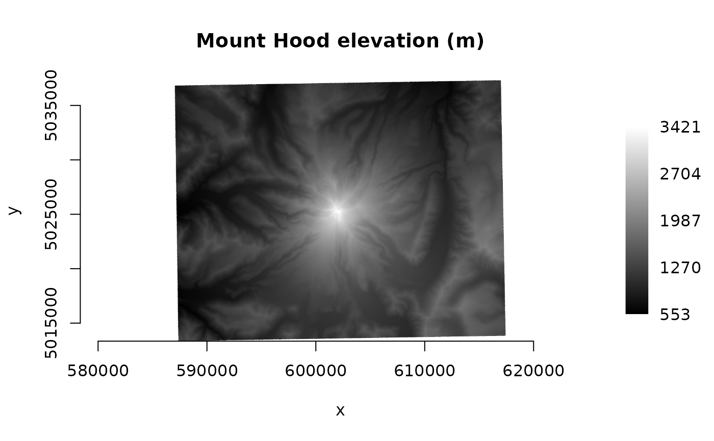
pal <- c("#00A60E", "#63C600", "#E6E600", "#E9BD3B", "#ECB176", "#EFC2B3",
         "#F2F2F2")

plot_raster(ds, legend = TRUE, col_map_fn = pal,
            main = "Mount Hood elevation (m)")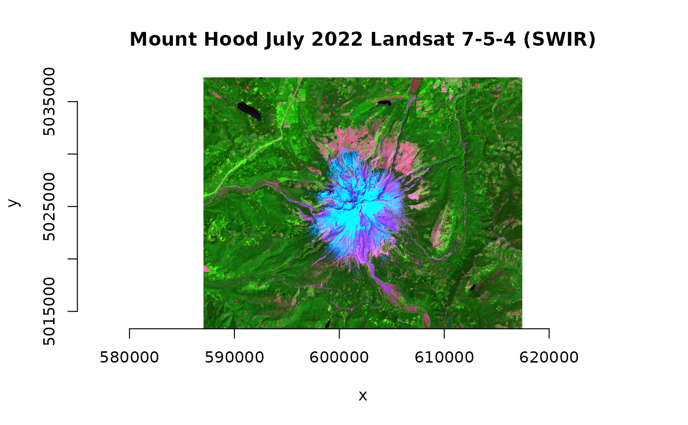
ds$close()RGB
f <- paste0(base_url, "landsat_c2ard_sr_mt_hood_jul2022_utm.tif")
ds <- new(GDALRaster, f)

# passing a vector of pixel values rather than the open dataset
r <- read_ds(ds, bands = c(7, 5, 4))
ds$close()

# normalizing to ranges derived from the full Landsat scene (2-98 percentiles)
plot_raster(r, minmax_def = c(7551,7679,7585,14842,24997,12451),
            main = "Mount Hood July 2022 Landsat 7-5-4 (SWIR)")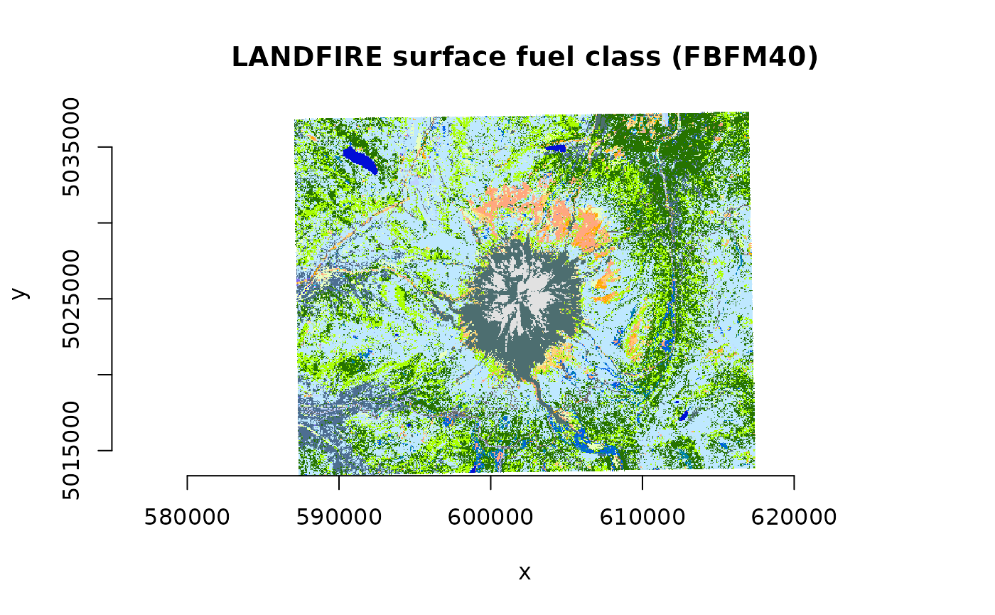
Color table
f <- paste0(base_url, "lf_fbfm40_220_mt_hood_utm.tif")
ds <- new(GDALRaster, f)
dm <- ds$dim()
paste("Size is", dm[1], "x",  dm[2], "x", dm[3])
#> [1] "Size is 1013 x 799 x 1"

# using the CSV attribute table distributed by LANDFIRE
fbfm_csv <- system.file("extdata/LF20_F40_220.csv", package="gdalraster")
vat <- read.csv(fbfm_csv)
head(vat)
#>   VALUE FBFM40   R   G   B      RED    GREEN     BLUE
#> 1    91    NB1 104 104 104 0.407843 0.407843 0.407843
#> 2    92    NB2 225 225 225 0.882353 0.882353 0.882353
#> 3    93    NB3 255 237 237 1.000000 0.929412 0.929412
#> 4    98    NB8   0  14 214 0.000000 0.054902 0.839216
#> 5    99    NB9  77 110 112 0.301961 0.431373 0.439216
#> 6   101    GR1 255 235 190 1.000000 0.921569 0.745098
vat <- vat[, c(1,6:8)]

# read at reduced resolution for display
plot_raster(ds, xsize = dm[1] / 2, ysize = dm[2] / 2,
            col_tbl = vat, interpolate = FALSE,
            main = "LANDFIRE surface fuel class (FBFM40)")
ds$close()Axis labels
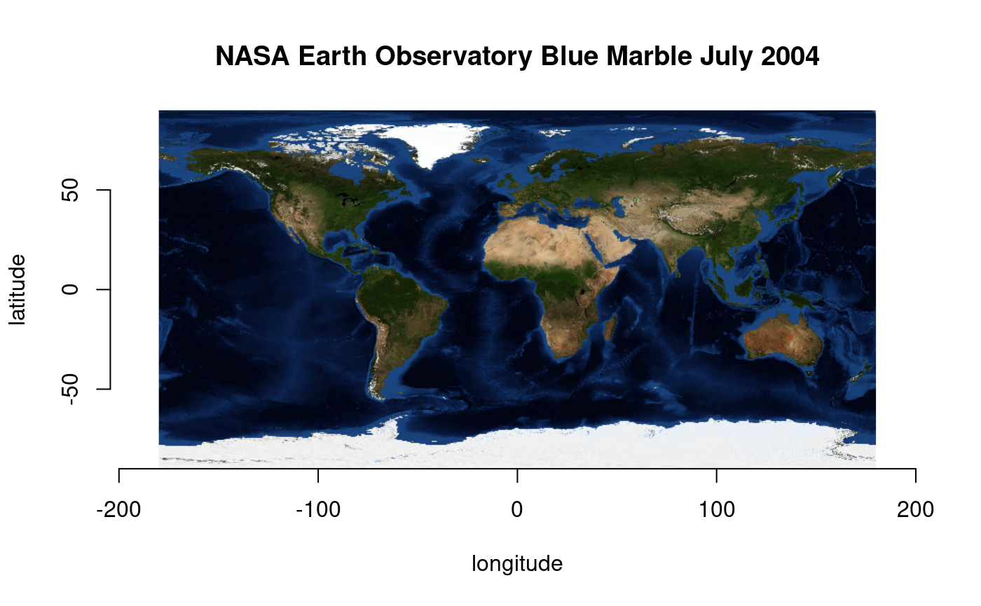
f <- paste0(base_url, "bl_mrbl_ng_jul2004_rgb_720x360.tif")
ds <- new(GDALRaster, f)
ds$getProjectionRef() |> srs_is_projected()
#> [1] FALSE
r <- read_ds(ds)
ds$close()

plot_raster(r, xlab = "longitude", ylab = "latitude",
            main = "NASA Earth Observatory Blue Marble July 2004")