Model-Assisted (MA) module overview
FIESTA’s Model-Assisted (MA) module calculates
population estimates and their sampling errors by taking advantage of
available model-assisted survey estimators from the mase R
package (McConville, et al. 2018). These estimators can use a variety of
auxiliary data to build models and predict over a response variable of
interest, while using a bias-correction term so that the bias of the
model does not depend on model misspecification.
Functions in FIESTA used for fitting model-assisted
estimators include the modMAarea function for area
estimates and modMAtree for tree estimates. The
modMApop function is used to get population data needed for
model-assisted estimation. Below is a description and table of contents
for the sections related to these functions:
| FUNCTION | DESCRIPTION |
|---|---|
| modMApop | Creates population data for model-assisted estimation. |
| modMAarea | Produces area level estimates through model-assisted estimation. |
| modMAtree | Produces tree level estimates through model-assisted estimation. |
Objective of tutorial
The main objective of this tutorial is to demonstrate how to use
FIESTA for generating estimates using estimators from
mase. The model-assisted estimators can be used with FIA’s
standard state-level population data (i.e, Evaluation) from the FIA
database (FIADB) and also population data from a custom boundary.
The following examples are for generating estimates and estimated
variances using standard FIA Evaluation data from FIA’s National
database, with custom Estimation unit and Stratification information.
The examples use data from three inventory years of field measurements
in the state of Wyoming, from FIADB_1.7.2.00, last updated June 20,
2018, downloaded on June 25, 2018 and stored as internal data objects in
FIESTA.
Example data - Wyoming (WY), Inventory Years 2011-2012
View MA Example Data
| Data Frame | Description |
|---|---|
| WYplt | WY plot-level data |
| WYcond | WY condition-level data |
| WYtree | WY tree-level data |
| External data | Description |
|---|---|
| WYbighorn_adminbnd.shp | Polygon shapefile of WY Bighorn National Forest Administrative boundary* |
| WYbighorn_districtbnd.shp | Polygon shapefile of WY Bighorn National Forest District boundaries** |
| WYbighorn_forest_nonforest_250m.tif | GeoTIFF raster of predicted forest/nonforest (1/0) for stratification*** |
| WYbighorn_dem_250m.img | Erdas Imagine raster of elevation change, in meters**** |
*USDA Forest Service, Automated Lands Program (ALP). 2018. S_USA.AdministrativeForest (http://data.fs.usda.gov/geodata/edw). Description: An area encompassing all the National Forest System lands administered by an administrative unit. The area encompasses private lands, other governmental agency lands, and may contain National Forest System lands within the proclaimed boundaries of another administrative unit. All National Forest System lands fall within one and only one Administrative Forest Area.
**USDA Forest Service, Automated Lands Program (ALP). 2018. S_USA.RangerDistrict (http://data.fs.usda.gov/geodata/edw). Description: A depiction of the boundary that encompasses a Ranger District.
***Based on MODIS-based classified map resampled from 250m to 500m resolution and reclassified from 3 to 2 classes: 1:forest; 2:nonforest. Projected in Albers Conical Equal Area, Datum NAD27 (Ruefenacht et al. 2008). Clipped to extent of WYbighorn_adminbnd.shp.
****USGS National Elevation Dataset (NED), resampled from 30m resolution to 250m. Projected in Albers Conical Equal Area, Datum NAD27 (U.S. Geological Survey 2017). Clipped to boundary of WYbighorn_adminbnd.shp.
Set up
First, you’ll need to load the FIESTA library:
Next, you’ll need to set up an “outfolder”. This is just a file path
to a folder where you’d like FIESTA to send your data
output. For this vignette, we have set our outfolder file path as a
temporary directory.
outfolder <- tempdir()Get data for examples
View Getting Data
Now that we’ve loaded FIESTA and setup our outfolder, we
can retrieve the data needed to run the examples. First, we point to
some external data and predictor layers stored in FIESTA
and derive new predictor layers using the terra
package.
# File names for external spatial data
WYbhfn <- system.file("extdata", "sp_data/WYbighorn_adminbnd.shp",
                      package = "FIESTA")

WYbhdistfn <- system.file("extdata", "sp_data/WYbighorn_districtbnd.shp",
                          package = "FIESTA")

## predictor variables
fornffn <- system.file("extdata", "sp_data/WYbighorn_forest_nonforest_250m.tif",
                       package = "FIESTA")

demfn <- system.file("extdata", "sp_data/WYbighorn_dem_250m.img",
                     package = "FIESTA")

# Derive new predictor layers from dem
library(terra)

dem <- rast(demfn)
slpfn <- paste0(outfolder, "/WYbh_slp.img")
slp <- terra::terrain(dem,
                      v = "slope",
                      unit = "degrees",
                      filename = slpfn,
                      overwrite = TRUE,
                      NAflag = -99999.0)

aspfn <- paste0(outfolder, "/WYbh_asp.img")
asp <- terra::terrain(dem,
                      v = "aspect",
                      unit = "degrees",
                      filename = aspfn,
                      overwrite = TRUE,
                      NAflag = -99999.0)
Next, we can get our FIA plot data and set up our auxiliary data. We
can get our FIA plot data with the spMakeSpatialPoints
function from FIESTA.
WYspplt <- spMakeSpatialPoints(xyplt = WYplt,
                               xy.uniqueid = "CN",
                               xvar = "LON_PUBLIC",
                               yvar = "LAT_PUBLIC",
                               xy.crs = 4269)

rastlst.cont <- c(demfn, slpfn, aspfn)
rastlst.cont.name <- c("dem", "slp", "asp")
rastlst.cat <- fornffn
rastlst.cat.name <- "fornf"
Next, we must prepare auxiliary data for model-assisted estimation.
We can do this with the spGetAuxiliary function from
FIESTA. See the sp vignette for further
information on this function.
modeldat <- spGetAuxiliary(xyplt = WYspplt,
                           uniqueid = "CN",
                           unit_layer = WYbhfn,
                           unitvar = NULL,
                           rastlst.cont = rastlst.cont,
                           rastlst.cont.name = rastlst.cont.name,
                           rastlst.cat = rastlst.cat,
                           rastlst.cat.name = rastlst.cat.name,
                           rastlst.cont.stat = "mean",
                           asptransform = TRUE,
                           rast.asp = aspfn,
                           keepNA = FALSE,
                           showext = FALSE,
                           savedata = FALSE)
str(modeldat, max.level = 1)output
## List of 12
##  $ unitvar       : chr "ONEUNIT"
##  $ pltassgn      :'data.frame':  56 obs. of  25 variables:
##  $ pltassgnid    : chr "CN"
##  $ unitarea      :'data.frame':  1 obs. of  2 variables:
##  $ areavar       : chr "ACRES_GIS"
##  $ unitzonal     :'data.frame':  1 obs. of  10 variables:
##  $ inputdf       :Classes 'data.table' and 'data.frame': 4 obs. of  7 variables:
##   ..- attr(*, ".internal.selfref")=<externalptr>
##  $ prednames     : chr [1:5] "dem" "slp" "asp_cos" "asp_sin" ...
##  $ zonalnames    : chr [1:7] "dem" "slp" "asp_cos" "asp_sin" ...
##  $ predfac       : chr "fornf"
##  $ npixelvar     : chr "npixels"
##  $ predfac.levels:List of 1
Examples
modMApop
Example 1: Creating our population dataset with
modMApop
View Example
We can create our population data for model-assisted estimation. To
do so, we use the modMApop function in FIESTA.
We must assign our population tables with the popTabs
argument (and unique identifiers for these tables with the
popTabIDs argument if they are not the default). Because we
used spGetAuxiliary to create our model data we can simply
pass the object returned by that function into the auxdat
argument in modMApop. This is a shortcut that allows you to
avoid manually specifying all of the necessary tables as function
arguments in modMApop.
MApopdat <- modMApop(popTabs = popTables(tree = WYtree,
                                         cond = WYcond,
                                         plt = WYplt),
                     auxdat = modeldat)
Note that the modMApop function returns a list with lots
of information and data for us to use. For a quick look at what this
list includes we can use the str function:
str(MApopdat, max.level = 1)output
## List of 40
##  $ module       : chr "MA"
##  $ popType      : chr "VOL"
##  $ pltidsadj    :Classes 'data.table' and 'data.frame':  56 obs. of  5 variables:
##   ..- attr(*, ".internal.selfref")=<externalptr>
##   ..- attr(*, "sorted")= Named chr "CN"
##   .. ..- attr(*, "names")= chr "CN"
##  $ pltcondx     :Classes 'data.table' and 'data.frame':  67 obs. of  40 variables:
##   ..- attr(*, ".internal.selfref")=<externalptr>
##   ..- attr(*, "sorted")= chr [1:2] "PLT_CN" "CONDID"
##  $ pltcondflds  : chr [1:39] "PLT_CN" "CONDID" "COND_NONSAMPLE_REASN_CD" "CONDPROP_UNADJ" ...
##  $ pjoinid      : Named chr "CN"
##   ..- attr(*, "names")= chr "CN"
##  $ cuniqueid    : chr "PLT_CN"
##  $ pltassgnid   : Named chr "CN"
##   ..- attr(*, "names")= chr "CN"
##  $ condid       : chr "CONDID"
##  $ ACI          : logi FALSE
##  $ areawt       : chr "CONDPROP_UNADJ"
##  $ areawt2      : NULL
##  $ adjcase      : Named chr "ADJ_FACTOR_COND"
##   ..- attr(*, "names")= chr "COND"
##  $ dbqueries    :List of 4
##  $ dbqueriesWITH:List of 4
##  $ pltassgnx    :Classes 'data.table' and 'data.frame':  56 obs. of  8 variables:
##   ..- attr(*, ".internal.selfref")=<externalptr>
##   ..- attr(*, "sorted")= Named chr "CN"
##   .. ..- attr(*, "names")= chr "CN"
##  $ unitlut      :Classes 'data.table' and 'data.frame':  1 obs. of  9 variables:
##   ..- attr(*, ".internal.selfref")=<externalptr>
##  $ unitarea     :Classes 'data.table' and 'data.frame':  1 obs. of  2 variables:
##   ..- attr(*, ".internal.selfref")=<externalptr>
##   ..- attr(*, "sorted")= chr "ONEUNIT"
##  $ npixels      :Classes 'data.table' and 'data.frame':  1 obs. of  2 variables:
##   ..- attr(*, ".internal.selfref")=<externalptr>
##  $ npixelvar    : chr "npixels"
##  $ estvar.area  : chr "CONDPROP_ADJ"
##  $ areavar      : chr "ACRES_GIS"
##  $ areaunits    : chr "acres"
##  $ unitvar      : chr "ONEUNIT"
##  $ unitvars     : chr "ONEUNIT"
##  $ plotsampcnt  :'data.frame':   2 obs. of  3 variables:
##  $ condsampcnt  :'data.frame':   4 obs. of  3 variables:
##  $ states       : chr "Wyoming"
##  $ invyrs       : int [1:3] 2011 2012 2013
##  $ adj          : chr "plot"
##  $ P2POINTCNT   :'data.frame':   0 obs. of  0 variables
##  $ plotunitcnt  :'data.frame':   1 obs. of  4 variables:
##  $ treex        :Classes 'data.table' and 'data.frame':  1706 obs. of  19 variables:
##   ..- attr(*, ".internal.selfref")=<externalptr>
##   ..- attr(*, "sorted")= chr [1:4] "PLT_CN" "CONDID" "SUBP" "TREE"
##  $ tuniqueid    : chr "PLT_CN"
##  $ adjtree      : logi FALSE
##  $ adjfactors   :Classes 'data.table' and 'data.frame':  56 obs. of  5 variables:
##   ..- attr(*, ".internal.selfref")=<externalptr>
##   ..- attr(*, "sorted")= Named chr "CN"
##   .. ..- attr(*, "names")= chr "CN"
##  $ adjvarlst    : Named chr [1:4] "ADJ_FACTOR_COND" "ADJ_FACTOR_SUBP" "ADJ_FACTOR_MACR" "ADJ_FACTOR_MICR"
##   ..- attr(*, "names")= chr [1:4] "COND" "SUBP" "MACR" "MICR"
##  $ prednames    : chr [1:5] "dem" "slp" "asp_cos" "asp_sin" ...
##  $ predfac      : chr "fornf"
##  $ popdatindb   : logi FALSE
Now that we’ve created our population data set, we can move on to estimation.
modMAarea
Example 2: Area of forest land, Wyoming, 2011-2013
View Example
In this example, we look at estimating the area of forest land in
Wyoming from 2011 to 2013 with the generalized regression estimator
(MAmethod = "greg"). We can specify a set of auxiliary
variables that we want to use in the model using the
prednames argument.
area1 <- modMAarea(MApopdat = MApopdat,             # pop - population calculations for WY
                   MAmethod = "greg",               # est - model-assisted method
                   prednames = c("dem", "fornf"),   # est - predictors to use in model
                   landarea = "FOREST")             # est - forest land filter
We can look at the structure of this output with str and
the estimates below. Note that again FIESTA outputs a
list.
str(area1, max.level = 2)output
## List of 5
##  $ est    :'data.frame': 1 obs. of  3 variables:
##   ..$ ONEUNIT               : chr "1"
##   ..$ Estimate              : num 1029015
##   ..$ Percent Sampling Error: num 3.93
##  $ raw    :List of 10
##   ..$ unit_totest  :'data.frame':    1 obs. of  17 variables:
##   ..$ domdat       :'data.frame':    40 obs. of  4 variables:
##   ..$ plotweights  :Classes 'data.table' and 'data.frame':   37 obs. of  5 variables:
##   .. ..- attr(*, ".internal.selfref")=<externalptr>
##   ..$ module       : chr "MA"
##   ..$ esttype      : chr "AREA"
##   ..$ MAmethod     : chr "greg"
##   ..$ predselectlst:List of 1
##   ..$ rowvar       : chr "TOTAL"
##   ..$ colvar       : chr "NONE"
##   ..$ areaunits    : chr "acres"
##  $ statecd: int 56
##  $ states : chr "Wyoming"
##  $ invyr  : int [1:3] 2011 2012 2013
area1$estoutput
##   ONEUNIT Estimate Percent Sampling Error
## 1       1  1029015                   3.93
Example 3: Area of forest land, Wyoming, 2011-2013, using the Elastic Net for variable selection
View Example
Here, we fit the same model as the above example, but we don’t
specify predictors and instead include modelselect = TRUE
which internally uses an elastic net model for variable selection.
area2 <- modMAarea(MApopdat = MApopdat,          # pop - population calculations for WY
                   MAmethod = "greg",
                   modelselect = TRUE,           # est - model-assisted method
                   landarea = "FOREST")          # est - forest land filter
We can again see that the structure of the list is very similar to that in the above example:
str(area2, max.level = 2)output
## List of 5
##  $ est    :'data.frame': 1 obs. of  3 variables:
##   ..$ ONEUNIT               : chr "1"
##   ..$ Estimate              : num 1036942
##   ..$ Percent Sampling Error: num 3.76
##  $ raw    :List of 11
##   ..$ unit_totest       :'data.frame':   1 obs. of  17 variables:
##   ..$ domdat            :'data.frame':   40 obs. of  4 variables:
##   ..$ plotweights       :Classes 'data.table' and 'data.frame':  37 obs. of  5 variables:
##   .. ..- attr(*, ".internal.selfref")=<externalptr>
##   ..$ module            : chr "MA"
##   ..$ esttype           : chr "AREA"
##   ..$ MAmethod          : chr "greg"
##   ..$ predselectlst     :List of 1
##   ..$ predselect.overall:Classes 'data.table' and 'data.frame':  1 obs. of  5 variables:
##   .. ..- attr(*, ".internal.selfref")=<externalptr>
##   ..$ rowvar            : chr "TOTAL"
##   ..$ colvar            : chr "NONE"
##   ..$ areaunits         : chr "acres"
##  $ statecd: int 56
##  $ states : chr "Wyoming"
##  $ invyr  : int [1:3] 2011 2012 2013
However now the raw list has an item called
predselectlst which stores information on the predictors
that were selected.
area2$raw$predselectlst$totestoutput
##    ONEUNIT TOTAL         dem       slp     asp_cos      asp_sin    fornf2
##     <fctr> <int>       <num>     <num>       <num>        <num>     <num>
## 1:       1     1 -0.04691924 0.0168218 -0.06238766 -0.008714709 0.0448006
And finally we can view the actual estimate:
area2$estoutput
##   ONEUNIT Estimate Percent Sampling Error
## 1       1  1036942                   3.76
Example 4: Area by forest type on forest land, Wyoming, 2011-2013
View Example
In this example, we look at adding rows to the output and include
returntitle = TRUE to return title information. Note that
when we do not explicitly supply prednames and do not set
modelselect to TRUE, FIESTA defaults to using all of the
available predictors.
area3 <- modMAarea(MApopdat = MApopdat,          # pop - population calculations for WY, post-stratification
                   MAmethod = "greg",            # est - model-assisted method
                   landarea = "FOREST",          # est - forest land filter
                   rowvar = "FORTYPCD",          # est - row domain
                   returntitle = TRUE)           # out - return title information
Again, we can look at the contents of the output list. The output now includes titlelst, a list of associated titles.
str(area3, max.level = 1)output
## List of 6
##  $ est     :'data.frame':    8 obs. of  3 variables:
##  $ titlelst:List of 10
##  $ raw     :List of 11
##  $ statecd : int 56
##  $ states  : chr "Wyoming"
##  $ invyr   : int [1:3] 2011 2012 2013
And the estimates:
area3$estoutput
##   Forest type Estimate Percent Sampling Error
## 1         201  44286.4                   85.2
## 2         265  89101.3                  52.03
## 3         266  97017.3                   42.4
## 4         268 112697.6                  34.19
## 5         281 618425.6                  13.59
## 6         901  38648.7                  75.39
## 7         999    36765                  64.92
## 8       Total  1036942                   3.76
Along with raw data and titles:
raw3 <- area3$raw      # extract raw data list object from output
names(raw3)
output
##  [1] "unit_totest"   "unit_rowest"   "domdat"        "plotweights"
##  [5] "module"        "esttype"       "MAmethod"      "predselectlst"
##  [9] "rowvar"        "colvar"        "areaunits"
head(raw3$unit_totest) # estimates by estimation unit (i.e., ESTN_UNIT)output
##   ONEUNIT      nhat    nhat.var NBRPLT NBRPLT.gt0 AREAUSED     est    est.var
## 1       1 0.9321562 0.001228216     37         37  1112412 1036942 1519869489
##    est.se     est.cv      pse CI99left CI99right CI95left CI95right CI68left
## 1 38985.5 0.03759661 3.759661   936522   1137362 960531.9   1113352 998172.6
##   CI68right
## 1   1075711
head(raw3$unit_rowest) # estimates by row, by estimation unit (i.e., ESTN_UNIT)output
##   ONEUNIT Forest type       nhat     nhat.var NBRPLT NBRPLT.gt0 AREAUSED
## 1       1         201 0.03981113 0.0011505987     37          2  1112412
## 2       1         265 0.08009738 0.0017367503     37          4  1112412
## 3       1         266 0.08721348 0.0013673266     37          5  1112412
## 4       1         268 0.10130923 0.0012000844     37          3  1112412
## 5       1         281 0.55593198 0.0057107487     37         23  1112412
## 6       1         901 0.03474316 0.0006861348     37          1  1112412
##         est    est.var   est.se    est.cv      pse  CI99left CI99right
## 1  44286.39 1423821285 37733.56 0.8520351 85.20351      0.00  141481.6
## 2  89101.31 2149161132 46359.05 0.5202959 52.02959      0.00  208514.3
## 3  97017.35 1692013618 41134.09 0.4239870 42.39870      0.00  202971.7
## 4 112697.64 1485057928 38536.45 0.3419455 34.19455  13434.33  211961.0
## 5 618425.60 7066830141 84064.44 0.1359330 13.59330 401889.95  834961.3
## 6  38648.72  849065242 29138.72 0.7539376 75.39376      0.00  113705.1
##    CI95left CI95right   CI68left CI68right
## 1      0.00 118242.80   6761.956  81810.82
## 2      0.00 179963.37  42999.193 135203.43
## 3  16396.01 177638.69  56111.224 137923.47
## 4  37167.59 188227.70  74374.767 151020.52
## 5 453662.33 783188.88 534827.056 702024.15
## 6      0.00  95759.57   9671.489  67625.96
# Titles (list object) for estimate
titlelst3 <- area3$titlelst
names(titlelst3)
output
##  [1] "title.est"     "title.pse"     "title.unitvar" "title.ref"
##  [5] "outfn.estpse"  "outfn.rawdat"  "outfn.param"   "title.rowvar"
##  [9] "title.row"     "title.unit"
titlelst3output
## $title.est
## [1] "Area, in acres, on forest land by forest type"
##
## $title.pse
## [1] "Percent sampling error of area, in acres, on forest land by forest type"
##
## $title.unitvar
## [1] "ONEUNIT"
##
## $title.ref
## [1] "Wyoming, 2011-2013"
##
## $outfn.estpse
## [1] "area_FORTYPCD_forestland"
##
## $outfn.rawdat
## [1] "area_FORTYPCD_forestland_rawdata"
##
## $outfn.param
## [1] "area_FORTYPCD_forestland_parameters"
##
## $title.rowvar
## [1] "Forest type"
##
## $title.row
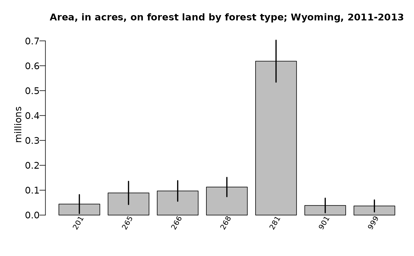
## [1] "Area, in acres, on forest land by forest type; Wyoming, 2011-2013"
##
## $title.unit
## [1] "acres"Example 5: Area by forest type and stand-size class on forest land, Wyoming, 2011-2013
View Example
In this example, we look at adding rows and columns to output,
including FIA names. We also output estimates and percent standard error
in the same cell with the allin1 argument in
table_options and save data to an outfolder with the
outfolder argument in savedata_options.
area4 <- modMAarea(MApopdat = MApopdat,                 # pop - population calculations for WY, post-stratification
                   MAmethod = "greg",                   # est - model-assisted method
                   landarea = "FOREST",                 # est - forest land filter
                   rowvar = "FORTYPCD",                 # est - row domain
                   colvar = "STDSZCD",                  # est - column domain
                   savedata = TRUE,                     # out - save data to outfolder
                   returntitle = TRUE,                  # out - return title information
                   table_opts = table_options(
                     row.FIAname = TRUE,                # table - row domain names
                     col.FIAname = TRUE,                # table - column domain names
                     allin1 = TRUE                      # table - return output with est(pse)
                   ),
                   savedata_opts = savedata_options(
                     outfolder = outfolder,             # save - outfolder for saving data
                     outfn.pre = "WY"                   # save - prefix for output files
                   ))
We can again look at the output list, estimates, raw data, and titles:
# Look at output list
names(area4)
output
## [1] "est" "pse" "titlelst" "raw" "statecd" "states" "invyr"
# Estimate and percent sampling error of estimate
head(area4$est)
output
##                        Forest type      Large diameter     Medium diameter
## 1                      Douglas-fir  28,381.5 (  95.01)        -- (     --)
## 2                 Engelmann spruce  97,387.6 (  40.28)  -8,286.3 (-339.39)
## 3 Engelmann spruce / subalpine fir  42,290.6 (  91.23)  28,627.2 (  48.64)
## 4                    Subalpine fir  36,053.1 (  81.54)        -- (     --)
## 5                   Lodgepole pine 221,069.2 (  28.62) 289,086.8 (  20.06)
## 6                            Aspen        -- (     --)        -- (     --)
##        Small diameter   Nonstocked               Total
## 1  15,904.9 ( 179.36) -- (     --)  44,286.4 (  85.20)
## 2        -- (     --) -- (     --)  89,101.3 (  52.03)
## 3  26,099.5 (  65.28) -- (     --)  97,017.3 (  42.40)
## 4  76,644.6 (  33.27) -- (     --) 112,697.6 (  34.19)
## 5 108,269.6 (  35.83) -- (     --) 618,425.6 (  13.59)
## 6  38,648.7 (  75.39) -- (     --)  38,648.7 (  75.39)
# Raw data (list object) for estimate
raw4 <- area4$raw      # extract raw data list object from output
names(raw4)
output
##  [1] "unit_totest"   "unit_rowest"   "unit_colest"   "unit_grpest"
##  [5] "domdat"        "plotweights"   "module"        "esttype"
##  [9] "MAmethod"      "predselectlst" "rowvar"        "colvar"
## [13] "areaunits"
head(raw4$unit_totest) # estimates by estimation unit (i.e., ESTN_UNIT)output
##   ONEUNIT      nhat    nhat.var NBRPLT NBRPLT.gt0 AREAUSED     est    est.var
## 1       1 0.9321562 0.001228216     37         37  1112412 1036942 1519869489
##    est.se     est.cv      pse CI99left CI99right CI95left CI95right CI68left
## 1 38985.5 0.03759661 3.759661   936522   1137362 960531.9   1113352 998172.6
##   CI68right
## 1   1075711
head(raw4$unit_rowest) # estimates by row, by estimation unit (i.e., ESTN_UNIT)output
##   ONEUNIT FORTYPCD       nhat     nhat.var NBRPLT NBRPLT.gt0
## 1       1      201 0.03981113 0.0011505987     37          2
## 2       1      265 0.08009738 0.0017367503     37          4
## 3       1      266 0.08721348 0.0013673266     37          5
## 4       1      268 0.10130923 0.0012000844     37          3
## 5       1      281 0.55593198 0.0057107487     37         23
## 6       1      901 0.03474316 0.0006861348     37          1
##                        Forest type AREAUSED       est    est.var   est.se
## 1                      Douglas-fir  1112412  44286.39 1423821285 37733.56
## 2                 Engelmann spruce  1112412  89101.31 2149161132 46359.05
## 3 Engelmann spruce / subalpine fir  1112412  97017.35 1692013618 41134.09
## 4                    Subalpine fir  1112412 112697.64 1485057928 38536.45
## 5                   Lodgepole pine  1112412 618425.60 7066830141 84064.44
## 6                            Aspen  1112412  38648.72  849065242 29138.72
##      est.cv      pse  CI99left CI99right  CI95left CI95right   CI68left
## 1 0.8520351 85.20351      0.00  141481.6      0.00 118242.80   6761.956
## 2 0.5202959 52.02959      0.00  208514.3      0.00 179963.37  42999.193
## 3 0.4239870 42.39870      0.00  202971.7  16396.01 177638.69  56111.224
## 4 0.3419455 34.19455  13434.33  211961.0  37167.59 188227.70  74374.767
## 5 0.1359330 13.59330 401889.95  834961.3 453662.33 783188.88 534827.056
## 6 0.7539376 75.39376      0.00  113705.1      0.00  95759.57   9671.489
##   CI68right
## 1  81810.82
## 2 135203.43
## 3 137923.47
## 4 151020.52
## 5 702024.15
## 6  67625.96
head(raw4$unit_colest) # estimates by column, by estimation unit (i.e., ESTN_UNIT)output
##   ONEUNIT STDSZCD       nhat     nhat.var NBRPLT NBRPLT.gt0 Stand-size class
## 1       1       1 0.38221627 0.0033901272     37         18   Large diameter
## 2       1       2 0.27815912 0.0030155927     37         14  Medium diameter
## 3       1       3 0.23873097 0.0024143561     37          6   Small diameter
## 4       1       5 0.03304982 0.0004603932     37          1       Nonstocked
##   AREAUSED       est    est.var   est.se    est.cv      pse CI99left CI99right
## 1  1112412 425182.10 4195150958 64769.99 0.1523347 15.23347 258345.7 592018.52
## 2  1112412 309427.64 3731679124 61087.47 0.1974209 19.74209 152076.7 466778.53
## 3  1112412 265567.28 2987672110 54659.60 0.2058220 20.58220 124773.5 406361.09
## 4  1112412  36765.03  569718693 23868.78 0.6492251 64.92251      0.0  98246.94
##   CI95left CI95right  CI68left CI68right
## 1 298235.3 552128.93 360771.07 489593.12
## 2 189698.4 429156.88 248678.72 370176.55
## 3 158436.4 372698.13 211210.61 319923.96
## 4      0.0  83546.98  13028.53  60501.53
head(raw4$unit_grpest) # estimates by row and column, by estimation unit (i.e., ESTN_UNIT)output
##   ONEUNIT grpvar         nhat     nhat.var NBRPLT NBRPLT.gt0 FORTYPCD STDSZCD
## 1       1  201#1  0.025513469 0.0005875578     37          1      201       1
## 2       1  201#3  0.014297657 0.0006576539     37          1      201       3
## 3       1  265#1  0.087546327 0.0012436962     37          3      265       1
## 4       1  265#2 -0.007448949 0.0006391340     37          1      265       2
## 5       1  266#1  0.038017056 0.0012029502     37          3      266       1
## 6       1  266#2  0.025734305 0.0001566975     37          1      266       2
##   Stand-size class                      Forest type AREAUSED       est
## 1   Large diameter                      Douglas-fir  1112412 28381.499
## 2   Small diameter                      Douglas-fir  1112412 15904.890
## 3   Large diameter                 Engelmann spruce  1112412 97387.615
## 4  Medium diameter                 Engelmann spruce  1112412 -8286.303
## 5   Large diameter Engelmann spruce / subalpine fir  1112412 42290.643
## 6  Medium diameter Engelmann spruce / subalpine fir  1112412 28627.159
##      est.var   est.se     est.cv        pse CI99left CI99right  CI95left
## 1  727079950 26964.42  0.9500703   95.00703        0  97837.24     0.000
## 2  813821229 28527.55  1.7936340  179.36340        0  89386.99     0.000
## 3 1539025822 39230.42  0.4028276   40.28276        0 198438.48 20497.406
## 4  790903534 28123.01 -3.3939149 -339.39149        0  64153.76     0.000
## 5 1488604221 38582.43  0.9123161   91.23161        0 141672.41     0.000
## 6  193907140 13925.05  0.4864281   48.64281        0  64495.72  1334.554
##   CI95right  CI68left CI68right
## 1  81230.79  1566.518  55196.48
## 2  71817.86     0.000  44274.34
## 3 174277.82 58374.615 136400.62
## 4  46833.78     0.000  19680.84
## 5 117910.82  3922.037  80659.25
## 6  55919.76 14779.279  42475.04
# Titles (list object) for estimate
titlelst4 <- area4$titlelst
names(titlelst4)
output
##  [1] "title.estpse"  "title.unitvar" "title.ref"     "outfn.estpse"
##  [5] "outfn.rawdat"  "outfn.param"   "title.rowvar"  "title.row"
##  [9] "title.colvar"  "title.col"     "title.unit"
titlelst4output
## $title.estpse
## [1] "Area, in acres (percent sampling error), by forest type and stand-size class on forest land"
##
## $title.unitvar
## [1] "ONEUNIT"
##
## $title.ref
## [1] "Wyoming, 2011-2013"
##
## $outfn.estpse
## [1] "WY_area_FORTYPCD_STDSZCD_forestland"
##
## $outfn.rawdat
## [1] "WY_area_FORTYPCD_STDSZCD_forestland_rawdata"
##
## $outfn.param
## [1] "WY_area_FORTYPCD_STDSZCD_forestland_parameters"
##
## $title.rowvar
## [1] "Forest type"
##
## $title.row
## [1] "Area, in acres (percent sampling error), by forest type on forest land; Wyoming, 2011-2013"
##
## $title.colvar
## [1] "Stand-size class"
##
## $title.col
## [1] "Area, in acres (percent sampling error), by stand-size class on forest land; Wyoming, 2011-2013"
##
## $title.unit
## [1] "acres"
# List output files in outfolder
list.files(outfolder, pattern = "WY_area")
output
## [1] "WY_area_FORTYPCD_STDSZCD_forestland_modMA_mase_greg.csv"
list.files(paste0(outfolder, "/rawdata"), pattern = "WY_area")output
## [1] "WY_area_FORTYPCD_STDSZCD_forestland_rawdata_modMA_mase_greg_domdat.csv"
## [2] "WY_area_FORTYPCD_STDSZCD_forestland_rawdata_modMA_mase_greg_plotweights.csv"
## [3] "WY_area_FORTYPCD_STDSZCD_forestland_rawdata_modMA_mase_greg_unit_colest.csv"
## [4] "WY_area_FORTYPCD_STDSZCD_forestland_rawdata_modMA_mase_greg_unit_grpest.csv"
## [5] "WY_area_FORTYPCD_STDSZCD_forestland_rawdata_modMA_mase_greg_unit_rowest.csv"
## [6] "WY_area_FORTYPCD_STDSZCD_forestland_rawdata_modMA_mase_greg_unit_totest.csv"
modMAtree
We now transition to from generating estimates of area to estimates
of tree attributes using the modMAtree function. This
requires that we set our estimate variable and filter. We set
estvar to "VOLCFNET" for net cubic foot
volume, and filter with estvar.filter set to
"STATUSCD == 1" so we only consider live trees in our
estimation.
estvar <- "VOLCFNET"
live_trees <- "STATUSCD == 1"
Example 6: Net cubic-foot volume of live trees, Wyoming, 2011-2013
View Example
tree1 <- modMAtree(MApopdat = MApopdat,            # pop - population calculations
                   MAmethod = "greg",              # est - model-assisted method
                   landarea = "FOREST",            # est - forest land filter
                   prednames = c("dem", "fornf"),  # est - predictors to use in model
                   estvar = estvar,                # est - net cubic-foot volume
                   estvar.filter = live_trees,     # est - live trees only
                   returntitle = TRUE)             # out - return title information

tree1$est
output
##   ONEUNIT   Estimate Percent Sampling Error
## 1       1 1931700102                   11.2
Example 7: Net cubic-foot volume of live trees, Wyoming, 2011-2013, using the Elastic Net for variable selection
View Example
Here, we fit the same model as the above example, but rather than
using "greg" are our model-assisted method, we can use
"gregEN" where the EN stands for “elastic net”. The elastic
net performs variable selection for us, grabbing predictors it finds to
be most useful in the model.
tree2 <- modMAtree(MApopdat = MApopdat,            # pop - population calculations
                   MAmethod = "greg",              # est - model-assisted method
                   modelselect = TRUE,             # est - perform variable selection internally
                   landarea = "FOREST",            # est - forest land filter
                   estvar = estvar,                # est - net cubic-foot volume
                   estvar.filter = live_trees,     # est - live trees only
                   returntitle = TRUE)             # out - return title information
We can again see that the structure of the list is very similar to that in the above example:
str(tree2, max.level = 2)output
## List of 6
##  $ est     :'data.frame':    1 obs. of  3 variables:
##   ..$ ONEUNIT               : chr "1"
##   ..$ Estimate              : num 1.6e+09
##   ..$ Percent Sampling Error: num 11.6
##  $ titlelst:List of 10
##   ..$ title.estpse : chr "Net merchantable bole  wood volume of live trees (timber species at least 5 inch dia), in cubic feet, and perce"| __truncated__
##   ..$ title.yvar   : chr "Net volume, in cubic feet"
##   ..$ title.estvar : chr "Net merchantable bole  wood volume of live trees (timber species at least 5 inch dia)"
##   ..$ title.unitvar: chr "ONEUNIT"
##   ..$ title.ref    : chr "Wyoming, 2011-2013"
##   ..$ outfn.estpse : chr "tree_VOLCFNET_forestland"
##   ..$ outfn.rawdat : chr "tree_VOLCFNET_forestland_rawdata"
##   ..$ outfn.param  : chr "tree_VOLCFNET_forestland_parameters"
##   ..$ title.tot    : chr "Net merchantable bole  wood volume of live trees (timber species at least 5 inch dia), in cubic feet, on forest"| __truncated__
##   ..$ title.unit   : chr "cubic feet"
##  $ raw     :List of 14
##   ..$ unit_totest       :'data.frame':   1 obs. of  17 variables:
##   ..$ domdat            :'data.frame':   40 obs. of  5 variables:
##   ..$ plotweights       :Classes 'data.table' and 'data.frame':  37 obs. of  5 variables:
##   .. ..- attr(*, ".internal.selfref")=<externalptr>
##   ..$ estvar            : chr "VOLCFNET"
##   ..$ estvar.filter     : chr "STATUSCD == 1"
##   ..$ module            : chr "MA"
##   ..$ esttype           : chr "TREE"
##   ..$ MAmethod          : chr "greg"
##   ..$ predselect.overall:Classes 'data.table' and 'data.frame':  1 obs. of  5 variables:
##   .. ..- attr(*, ".internal.selfref")=<externalptr>
##   ..$ predselectlst     :List of 1
##   ..$ rowvar            : chr "TOTAL"
##   ..$ colvar            : chr "NONE"
##   ..$ areaunits         : chr "acres"
##   ..$ estunits          : chr "cubic feet"
##  $ statecd : int 56
##  $ states  : chr "Wyoming"
##  $ invyr   : int [1:3] 2011 2012 2013
However now the raw list has an item call
predselectlst. We can look at this item now:
tree2$raw$predselectlstoutput
## $totest
##    ONEUNIT TOTAL      dem       slp   asp_cos   asp_sin   fornf2
##     <fctr> <int>    <num>     <num>     <num>     <num>    <num>
## 1:       1     1 415.5025 -481.4989 -144.2504 -620.3723 -763.951
And finally, we can look at the estimate
tree2$estoutput
##   ONEUNIT   Estimate Percent Sampling Error
## 1       1 1602795606                  11.59
Example 8: Net cubic-foot volume of live trees by forest type, Wyoming, 2011-2013
View Example
This example adds rows to the output for net cubic-foot volume of
live trees (at least 5 inches diameter) by forest type, Wyoming,
2011-2013. We also choose to return titles with
returntitle = TRUE.
tree3 <- modMAtree(MApopdat = MApopdat,               # pop - population calculations
                   MAmethod = "greg",                 # est - model-assisted method
                   prednames = c("dem", "fornf"),     # est - predictors to use in model
                   landarea = "FOREST",               # est - forest land filter
                   estvar = "VOLCFNET",               # est - net cubic-foot volume
                   estvar.filter = "STATUSCD == 1",   # est - live trees only
                   rowvar = "FORTYPCD",               # est - row domain
                   returntitle = TRUE)                # out - return title information
Again, we investigate the output:
# Look at output list
names(tree3)
output
## [1] "est" "titlelst" "raw" "statecd" "states" "invyr"
# Estimate and percent sampling error of estimate
tree3$est
output
##   Forest type     Estimate Percent Sampling Error
## 1         201   14937765.2                  104.5
## 2         265  477236769.3                  38.99
## 3         266  202892988.5                  57.86
## 4         268   53707726.6                  90.31
## 5         281 1182924852.4                  18.33
## 6         901           --                     --
## 7         999           --                     --
## 8       Total   1931700102                   11.2
We can also create a simple barplot from the output:
datBarplot(raw3$unit_rowest,
           xvar = titlelst3$title.rowvar,
           yvar = "est")
plot

And a fancier barplot:
datBarplot(raw3$unit_rowest,
           xvar = titlelst3$title.rowvar,
           yvar = "est",
           errbars = TRUE,
           sevar = "est.se",
           main = FIESTAutils::wraptitle(titlelst3$title.row, 75),
           ylabel = titlelst3$title.yvar,
           divideby = "million")
plot
Example 9: Net cubic-foot volume of live trees by forest type and stand-size class, Wyoming, 2011-2013
View Example
This examples adds rows and columns to the output, including FIA
names, for net cubic-foot volume of live trees (at least 5 inches
diameter) by forest type and stand-size class, Wyoming, 2011-2013. We
also use the *_options functions to return output with
estimates (est) and percent standard error (pse) in same cell - est(pse)
with allin1 = TRUE and save data to an outfolder with
savedata = TRUE and outfolder = outfolder.
tree4 <- modMAtree(MApopdat = MApopdat,                # pop - population calculations
                   MAmethod = "greg",                  # est - model-assisted method
                   landarea = "FOREST",                # est - forest land filter
                   prednames = c("dem", "slp"),        # est - predictors to use in model
                   estvar = "VOLCFNET",                # est - net cubic-foot volume
                   estvar.filter = "STATUSCD  == 1",   # est - live trees only
                   rowvar = "FORTYPCD",                # est - row domain
                   colvar = "STDSZCD",                 # est - column domain
                   returntitle = TRUE,                 # out - return title information
                   savedata = TRUE,                    # out - save data to outfolder
                   table_opts = table_options(
                     row.FIAname = TRUE,               # est - row domain names
                     col.FIAname = TRUE,               # est - column domain names
                     allin1 = TRUE                     # out - return output with est(pse)
                   ),
                   savedata_opts = savedata_options(
                     outfolder = outfolder,            # out - outfolder for saving data
                     outfn.pre = "WY"                  # out - prefix for output files
                   ))
Again, we investigate the output of the returned list:
# Look at output list from modGBarea()
names(tree4)
output
## [1] "est" "pse" "titlelst" "raw" "statecd" "states" "invyr"
# Estimate and percent sampling error of estimate
tree4$est
output
##                        Forest type           Large diameter
## 1                      Douglas-fir    13,220,807.8 (110.84)
## 2                 Engelmann spruce   280,813,787.4 ( 56.81)
## 3 Engelmann spruce / subalpine fir   258,361,837.5 ( 46.33)
## 4                    Subalpine fir    64,151,931.3 ( 74.52)
## 5                   Lodgepole pine   843,091,898.5 ( 23.55)
## 6                            Aspen              -- (    --)
## 7                       Nonstocked              -- (    --)
## 8                            Total 1,459,640,262.5 ( 14.80)
##          Medium diameter        Small diameter  Nonstocked
## 1            -- (    --)  3,232,360.3 (162.26) -- (    --)
## 2  91,643,840.9 (115.58)           -- (    --) -- (    --)
## 3  19,870,297.1 ( 73.46)  6,039,623.3 ( 88.17) -- (    --)
## 4            -- (    --)           -- (    --) -- (    --)
## 5 423,496,333.8 ( 28.44) 11,122,841.6 ( 61.94) -- (    --)
## 6            -- (    --)           -- (    --) -- (    --)
## 7            -- (    --)           -- (    --) -- (    --)
## 8 535,010,471.8 ( 26.77) 20,394,825.1 ( 45.99) -- (    --)
##                      Total
## 1    16,453,168.1 ( 91.71)
## 2   372,457,628.3 ( 50.51)
## 3   284,271,757.8 ( 41.67)
## 4    64,151,931.3 ( 74.52)
## 5 1,277,711,073.9 ( 16.98)
## 6              -- (    --)
## 7              -- (    --)
## 8 2,015,045,559.4 ( 10.67)
## Raw data (list object) for estimate
raw4 <- tree4$raw      # extract raw data list object from output
names(raw4)
output
##  [1] "unit_totest"   "unit_rowest"   "unit_colest"   "unit_grpest"
##  [5] "domdat"        "plotweights"   "estvar"        "estvar.filter"
##  [9] "module"        "esttype"       "MAmethod"      "predselectlst"
## [13] "rowvar"        "colvar"        "areaunits"     "estunits"
head(raw4$unit_totest) # estimates by estimation unit (i.e., ESTN_UNIT)output
##   ONEUNIT    nhat nhat.var NBRPLT NBRPLT.gt0 AREAUSED        est      est.var
## 1       1 1811.42  37356.8     37         34  1112412 2015045559 4.622759e+16
##      est.se    est.cv      pse   CI99left  CI99right   CI95left  CI95right
## 1 215006029 0.1067003 10.67003 1461226728 2568864391 1593641485 2436449634
##     CI68left  CI68right
## 1 1801231118 2228860000
head(raw4$unit_rowest) # estimates by row, by estimation unit (i.e., ESTN_UNIT)output
##   ONEUNIT FORTYPCD       nhat   nhat.var NBRPLT NBRPLT.gt0
## 1       1      201   14.79053   183.9783     37          2
## 2       1      265  334.81975 28597.8813     37          4
## 3       1      266  255.54531 11338.6666     37          5
## 4       1      268   57.66920  1847.0547     37          2
## 5       1      281 1148.59483 38016.6026     37         23
## 6       1      901    0.00000     0.0000     37          0
##                        Forest type AREAUSED        est      est.var    est.se
## 1                      Douglas-fir  1112412   16453168 2.276660e+14  15088604
## 2                 Engelmann spruce  1112412  372457628 3.538877e+16 188119031
## 3 Engelmann spruce / subalpine fir  1112412  284271758 1.403116e+16 118453199
## 4                    Subalpine fir  1112412   64151931 2.285659e+15  47808562
## 5                   Lodgepole pine  1112412 1277711074 4.704407e+16 216896455
## 6                            Aspen  1112412          0 0.000000e+00         0
##      est.cv      pse  CI99left  CI99right  CI95left  CI95right   CI68left
## 1 0.9170637 91.70637         0   55318835         0   46026287    1448187
## 2 0.5050750 50.50750         0  857020140   3751103  741164153  185381175
## 3 0.4166900 41.66900         0  589386980  52107753  516435763  166475040
## 4 0.7452396 74.52396         0  187298626         0  157854990   16608330
## 5 0.1697539 16.97539 719022828 1836399319 852601833 1702820315 1062016684
## 6       NaN      NaN         0          0         0          0          0
##    CI68right
## 1   31458149
## 2  559534081
## 3  402068476
## 4  111695532
## 5 1493405464
## 6          0
head(raw4$unit_colest) # estimates by column, by estimation unit (i.e., ESTN_UNIT)output
##   ONEUNIT STDSZCD       nhat    nhat.var NBRPLT NBRPLT.gt0 Stand-size class
## 1       1       1 1312.13957 37720.24765     37         18   Large diameter
## 2       1       2  480.94618 16570.36181     37         14  Medium diameter
## 3       1       3   18.33387    71.08256     37          4   Small diameter
## 4       1       5    0.00000     0.00000     37          0       Nonstocked
##   AREAUSED        est      est.var    est.se    est.cv      pse  CI99left
## 1  1112412 1459640263 4.667734e+16 216049403 0.1480155 14.80155 903133879
## 2  1112412  535010472 2.050518e+16 143196301 0.2676514 26.76514 166161244
## 3  1112412   20394825 8.796191e+13   9378801 0.4598618 45.98618         0
## 4  1112412          0 0.000000e+00         0       NaN      NaN         0
##    CI99right   CI95left  CI95right   CI68left  CI68right
## 1 2016146646 1036191214 1883089311 1244788231 1674492295
## 2  903859699  254350880  815670064  392607782  677413162
## 3   44553016    2012713   38776937   11068003   29721648
## 4          0          0          0          0          0
head(raw4$unit_grpest) # estimates by row and column, by estimation unit (i.e., ESTN_UNIT)output
##   ONEUNIT grpvar       nhat    nhat.var NBRPLT NBRPLT.gt0 FORTYPCD STDSZCD
## 1       1  201#1  11.884809   173.51852     37          1      201       1
## 2       1  201#3   2.905721    22.22926     37          1      201       3
## 3       1  265#1 252.436776 20564.47714     37          3      265       1
## 4       1  265#2  82.382977  9067.00974     37          1      265       2
## 5       1  266#1 232.253657 11575.99347     37          3      266       1
## 6       1  266#2  17.862348   172.20105     37          1      266       2
##   Stand-size class                      Forest type AREAUSED       est
## 1   Large diameter                      Douglas-fir  1112412  13220808
## 2   Small diameter                      Douglas-fir  1112412   3232360
## 3   Large diameter                 Engelmann spruce  1112412 280813787
## 4  Medium diameter                 Engelmann spruce  1112412  91643841
## 5   Large diameter Engelmann spruce / subalpine fir  1112412 258361838
## 6  Medium diameter Engelmann spruce / subalpine fir  1112412  19870297
##        est.var    est.se    est.cv       pse CI99left CI99right CI95left
## 1 2.147224e+14  14653411 1.1083597 110.83597        0  50965492        0
## 2 2.750785e+13   5244793 1.6225891 162.25891        0  16742051        0
## 3 2.544774e+16 159523489 0.5680757  56.80757        0 691719064        0
## 4 1.122007e+16 105924847 1.1558316 115.58316        0 364488165        0
## 5 1.432484e+16 119686437 0.4632512  46.32512        0 566653670 23780731
## 6 2.130921e+14  14597675 0.7346481  73.46481        0  57471417        0
##   CI95right  CI68left CI68right
## 1  41940965         0  27793007
## 2  13511965         0   8448086
## 3 593474080 122174397 439453178
## 4 299252726         0 196981640
## 5 492942944 139338716 377384959
## 6  48481215   5353524  34387070
# Titles (list object) for estimate
titlelst4 <- tree4$titlelst
names(titlelst4)
output
##  [1] "title.estpse"  "title.yvar"    "title.estvar"  "title.unitvar"
##  [5] "title.ref"     "outfn.estpse"  "outfn.rawdat"  "outfn.param"
##  [9] "title.rowvar"  "title.row"     "title.colvar"  "title.col"
## [13] "title.unit"
titlelst4output
## $title.estpse
## [1] "Net merchantable bole  wood volume of live trees (timber species at least 5 inch dia), in cubic feet (percent sampling error), by forest type and stand-size class on forest land"
##
## $title.yvar
## [1] "Net volume, in cubic feet"
##
## $title.estvar
## [1] "Net merchantable bole  wood volume of live trees (timber species at least 5 inch dia)"
##
## $title.unitvar
## [1] "ONEUNIT"
##
## $title.ref
## [1] "Wyoming, 2011-2013"
##
## $outfn.estpse
## [1] "WY_tree_VOLCFNET_FORTYPCD_STDSZCD_forestland"
##
## $outfn.rawdat
## [1] "WY_tree_VOLCFNET_FORTYPCD_STDSZCD_forestland_rawdata"
##
## $outfn.param
## [1] "WY_tree_VOLCFNET_FORTYPCD_STDSZCD_forestland_parameters"
##
## $title.rowvar
## [1] "Forest type"
##
## $title.row
## [1] "Net merchantable bole  wood volume of live trees (timber species at least 5 inch dia), in cubic feet (percent sampling error), by forest type on forest land; Wyoming, 2011-2013"
##
## $title.colvar
## [1] "Stand-size class"
##
## $title.col
## [1] "Net merchantable bole  wood volume of live trees (timber species at least 5 inch dia), in cubic feet (percent sampling error), by stand-size class on forest land; Wyoming, 2011-2013"
##
## $title.unit
## [1] "cubic feet"
# List output files in outfolder
list.files(outfolder, pattern = "WY_tree")
output
## [1] "WY_tree_VOLCFNET_FORTYPCD_STDSZCD_forestland_modMA_mase_greg.csv"
list.files(paste0(outfolder, "/rawdata"), pattern = "WY_tree")output
## [1] "WY_tree_VOLCFNET_FORTYPCD_STDSZCD_forestland_rawdata_modMA_mase_greg_domdat.csv"
## [2] "WY_tree_VOLCFNET_FORTYPCD_STDSZCD_forestland_rawdata_modMA_mase_greg_plotweights.csv"
## [3] "WY_tree_VOLCFNET_FORTYPCD_STDSZCD_forestland_rawdata_modMA_mase_greg_unit_colest.csv"
## [4] "WY_tree_VOLCFNET_FORTYPCD_STDSZCD_forestland_rawdata_modMA_mase_greg_unit_grpest.csv"
## [5] "WY_tree_VOLCFNET_FORTYPCD_STDSZCD_forestland_rawdata_modMA_mase_greg_unit_rowest.csv"
## [6] "WY_tree_VOLCFNET_FORTYPCD_STDSZCD_forestland_rawdata_modMA_mase_greg_unit_totest.csv"
Example 10: Number of live trees (plus seedlings) by species, Wyoming, 2011-2013
View Example
We can also add seedlings.
Note: seedling data are only available for number of trees (estvar = TPA_UNADJ).
Note: must include seedling data in population data calculations.
MApopdat_seed <- modMApop(popTabs = popTables(tree = WYtree,
                                              cond = WYcond,
                                              seed = WYseed),
                          pltassgn = WYpltassgn,
                          auxdat = modeldat)
tree5 <- modMAtree(MApopdat = MApopdat_seed,              # pop - population calculations
                   MAmethod = "greg",                     # est - model-assisted method
                   prednames = c("dem", "slp", "fornf"),
                   estseed = "add",                       # est - add seedling data
                   landarea = "FOREST",                   # est - forest land filter
                   estvar = "TPA_UNADJ",                  # est - number of trees per acre
                   estvar.filter = "STATUSCD == 1",       # est - live trees only
                   rowvar = "SPCD",                       # est - row domain
                   returntitle = TRUE,                    # out - return title information
                   table_opts = table_options(
                     row.FIAname = TRUE,                  # est - row domain names
                     allin1 = FALSE                       # out - return output with est and pse
                   ))
And again we can look at our outputs and compare estimates:
# Look at output list
names(tree5)
output
## [1] "est" "titlelst" "raw" "statecd" "states"
# Estimate and percent sampling error of estimate
tree5$est
output
##                                Species     Estimate Percent Sampling Error
## 1     subalpine fir (Abies lasiocarpa)  790299214.1                  14.69
## 2 Engelmann spruce (Picea engelmannii)  259528743.9                  20.03
## 3      lodgepole pine (Pinus contorta)  311324152.7                  18.87
## 4         limber pine (Pinus flexilis)   41737320.1                 127.12
## 5  Douglas-fir (Pseudotsuga menziesii)   57576633.6                 102.22
## 6  quaking aspen (Populus tremuloides)   91703320.1                 107.42
## 7                                Total 1552169384.5                  12.85