FIA plots - species distribution map • FIESTA

The FIESTA R package is an estimation engine that generates estimates using FIA data for custom situations (Frescino et al. 2023). The package provides functions for using FIA’s standard estimation techniques and also includes different modules for using alternative estimation strategies for unique situations (Frescino et al. 2022). The package facilitates compilation of FIA and geospatial auxiliary information needed for estimation and provides consistent output for reporting.

To use the FIESTA R package, you need to be familiar with the R statistical software and also have a firm knowledge of the FIA database. Please consult the FIA database description user guide (Version 9.0.1) for variable descriptions (Burrill et al. 2021).

The following examples demonstrate how we use FIESTA for compiling plot-level summaries.

Setup

First install the necessary packages and define outfolders.

options(scipen = 6)
library(FIESTA)

Next we can specify a few parameters:

spcd <- c(101, 113)
tfilter <- FIESTAutils::getfilter("SPCD", spcd)

We can look at the resulting filter and use the internal ref_species table to decide on a name for the column in the output data frame.

tfilter

## [1] "SPCD %in% c(101, 113)"

ref <- ref_species[ref_species$SPCD %in% spcd, ]
ref

##      SPCD    COMMON_NAME GENUS    SPECIES VARIETY SUBSPECIES SPECIES_SYMBOL
## 1595  113    limber pine Pinus   flexilis    <NA>       <NA>          PIFL2
## 2029  101 whitebark pine Pinus albicaulis    <NA>       <NA>           PIAL
##      E_SPGRPCD W_SPGRPCD C_SPGRPCD P_SPGRPCD WOODLAND SFTWD_HRDWD MAJOR_SPGRPCD
## 1595         9        24        NA        NA        N           S             1
## 2029         9        24        NA        NA        N           S             1
##      JENKINS_TOTAL_B1 JENKINS_TOTAL_B2 DRYWT_TO_GREENWT_CONVERSION
## 1595          -2.5356           2.4349                    1.822335
## 2029          -2.5356           2.4349                    1.751189
##      CARBON_RATIO_LIVE MODIFIED_DATE  SCIENTIFIC_NAME
## 1595             0.480    2023-05-25   Pinus flexilis
## 2029             0.478    2023-05-25 Pinus albicaulis

spcd_name <- "whitebark_limber"

Finally we create a spatial points data frame using the internal Wyoming plot data

WYpltsp <- spMakeSpatialPoints(xyplt = WYplt,
                               xy.uniqueid = "CN",
                               xvar = "LON_PUBLIC",
                               yvar = "LAT_PUBLIC")

Summarize Plots

Finally we can put all of the pieces together to get plot level species presence/absence:

pltdomdat <- datSumTreeDom(plt = WYpltsp,
                           tree = WYtree,
                           seed = WYseed,
                           bycond = FALSE,
                           tsumvar = "TPA_UNADJ",
                           tfilter = tfilter,
                           tdomtot = TRUE,
                           tdomtotnm = spcd_name,
                           seedlings = "Y",
                           presence = TRUE,
                           FIAname = TRUE,
                           datSum_opts = list(keepall = TRUE))

tdomdat.pres <- pltdomdat$tdomdat.pres
head(tdomdat.pres)

## Simple feature collection with 6 features and 22 fields
## Geometry type: POINT
## Dimension:     XY
## Bounding box:  xmin: -106.0363 ymin: 42.26546 xmax: -105.6679 ymax: 42.41013
## Geodetic CRS:  NAD83
##               CN INVYR STATECD CYCLE UNITCD COUNTYCD  PLOT MEASYEAR RDDISTCD
## 1 40404728010690  2013      56     3      2        1 86688     2013       NA
## 2 40404729010690  2011      56     3      2        1 84596     2011        1
## 3 40404730010690  2013      56     3      2        1 88993     2013        6
## 4 40404731010690  2012      56     3      2        1 82340     2012       NA
## 5 40404733010690  2012      56     3      2        1 82869     2012       NA
## 6 40404734010690  2013      56     3      2        1 83304     2013       NA
##   NF_SAMPLING_STATUS_CD PLOT_STATUS_CD NF_PLOT_STATUS_CD NBRCND NBRCNDSAMP
## 1                     0              2                NA      1          1
## 2                     0              1                NA      1          1
## 3                     0              1                NA      1          1
## 4                     0              2                NA      1          1
## 5                     0              2                NA      1          1
## 6                     0              2                NA      1          1
##   NBRCNDFOR CCLIVEPLT        FORNONSAMP        PLOT_ID SPCD whitebark pine
## 1         0         0 Sampled-Nonforest ID560200186688   NA              0
## 2         1        17    Sampled-Forest ID560200184596  113              0
## 3         1        41    Sampled-Forest ID560200188993  113              0
## 4         0         0 Sampled-Nonforest ID560200182340   NA              0
## 5         0         0 Sampled-Nonforest ID560200182869   NA              0
## 6         0         0 Sampled-Nonforest ID560200183304   NA              0
##   limber pine whitebark_limber                   geometry
## 1           0                0 POINT (-105.9625 42.41013)
## 2           1                1 POINT (-105.7277 42.40928)
## 3           1                1 POINT (-105.6679 42.40953)
## 4           0                0 POINT (-106.0313 42.35599)
## 5           0                0 POINT (-105.8509 42.31655)
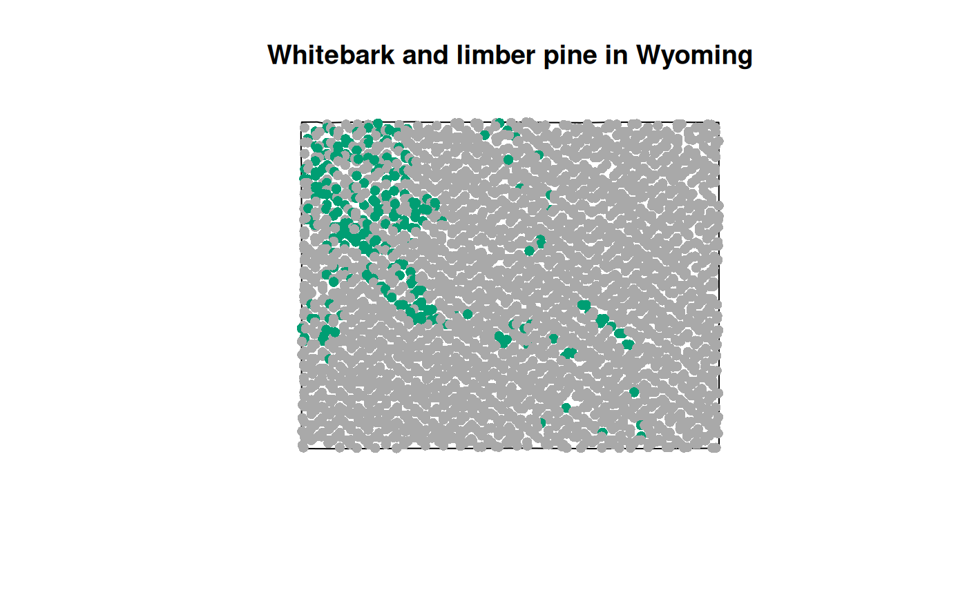
## 6           0                0 POINT (-106.0363 42.26546)

And we can plot the results to get a picture of the whitebark_limber presence/absence distribution.

cols <- c("0" = "darkgrey", "1" = "#009E73")
point_cols <- cols[as.character(tdomdat.pres$whitebark_limber)]

f <- system.file("extdata/sp_data/wy_bnd.gpkg", package = "FIESTA")
WYbnd <- sf::st_read(f, quiet = TRUE)

plot(sf::st_geometry(WYbnd), main = "Whitebark and limber pine in Wyoming")
plot(tdomdat.pres[ ,"whitebark_limber"], col = point_cols, pch = 16, add = TRUE)